Methods for decomposing time series data into trend and seasonality are incredibly powerful and useful, but sometimes suffer from an inability to act without some prior information from the algorithm user about the periodic nature of the seasonality. In this post we’re going to talk about a methodology, born from the world of signal processing, to automatically analyze and feed this additional information into decomposition algorithms to take that burden out of the hands of users!
Time Series Overview
Time series data differs from other machine learning dataset in one crucial way: they possess datetime information that provides structure and order to the data. Normally, this datetime data presents itself as an index of the data, in ascending order where individual rows represent samplings of each of the feature columns for that specific datetime. For single series problems, representing measurements of say one system, one product SKU, one patient, etc. the datetime values are unique with one measurement or vector of measurements per datetime value. For univariate time series problems, we seek to model a single target variable and take advantage of the common methodology of breaking that target value into three components: a trend-cycle component, a seasonality component and the residual component.

Trend and Seasonality Overview
Hyndman covers the theory behind trend and seasonality decomposition quite well in his Forecasting textbook, freely available online. The gist is that a target series can be broken either a sum or a product of three series: the trend-cycle, the seasonality and the residual.
The trend-cycle, commonly just called the trend, captures the longer-term motion of the target value. Think of the general, upward rise in the Dow Jones index.

The seasonality captures repeating, periodic motion in the target value. This is readily visible in natural datasets with some dependency on the rotation or tilt of the earth, like the daily temperatures in Melbourne, Australia.

The residual is just what’s left over after the trend and seasonality have been removed from the target series. The residual can be formed by either subtracting out or dividing out the calculated trend and seasonality, depending on whether the target is assessed to have additive or multiplicative trend and seasonality respectively.
There are a variety of industry standard approaches to decomposing a target signal into trend, seasonality and residual. STL is an extremely common one, but also popular in certain circles are X11 and X13. The result looks something like this:

Utilizing Trend and Seasonality Decomposition in Auto ML
From an engineering and auto ML perspective, we like to attempt decomposition of all time series datasets prior to modeling them. A successful decomposition of the target data into these three components can make the modeling process significantly easier and more accurate. Identifying and separating out the trend and seasonal components and modeling the residual can be thought of as reducing the cognitive load on the ML algorithms, letting them focus on the trickier patterns in the data without being distracted by the larger, obvious signals.
One challenge in trend and seasonality decomposition is that one most know before performing the decomposition what the period of the seasonal signal is! This can be demoralizing as neophytes into the world of time series decomposition might expect modern libraries that execute seasonal decomposition to do this for them. Sadly, that is not the case. For seasoned data scientists and machine learning practitioners working on a single study, part of their workflow is to determine the period of that signal and they have Jupyter notebooks aplenty rife with meticulously written cells of complicated code to do so. But what about those that want to gain the insights of trend and seasonality decomposition without that time or ability?
Fortunately, the detection of periodicity within a target series and a good first guess at the period is not particularly challenging. This is all thanks to a commonly used technique called autocorrelation.
Autocorrelation
To discuss autocorrelation, which is the correlation of a signal with itself, it’s important to first discuss correlation and dip into the world of signals processing. Correlation is the convolution of one signal in time with the functional inverse of the other. So, let’s start with convolution.
A convolution can be intuitively understood as the continuous multiplication and summation of two signals overlayed on top of one another. Mathematically, convolution looks like:


If we look at the animation of the convolution of two box signals, we notice the curious property that the peak of the convolution, (f * g)(t), is maximized at the location of the integral dummy variable 𝜏 during which the two signals overlap entirely.
Now how about the correlation? You’ll frequently see “correlation” and “cross-correlation” used interchangeably. Normally, “correlation” refers to “autocorrelation”, which is the correlation of a signal with itself, while “cross-correlation” refers to the correlation of a signal with a different signal.

Here, we see the cross-correlation of two signals, a box and a wedge. The animation shows the cross-correlation being executed by sliding a kernel, in this case the red wedge function, across a stationary reference of the blue box function, generating the resulting black cross-correlation function. Although this is a continuous integral operation, you can imagine infinitesimally shifting the kernel, multiplying the values of both red and blue functions together, summing those products and generating the cross-correlation at each value of t during the sliding operation.
You’re probably also wondering, why does cross-correlation and convolution look like the same operation? Well, in the convolution case, we were a bit cheeky in selecting two box signals to convolve. Technically, the second function in the convolution, the kernel, is flipped 180 degrees before the slide/multiply/sum operations take place.
Finally, let’s talk about the extension to the convolution concept that we use for period detection: autocorrelation. As we’ve said, autocorrelation is just the correlation of a signal with itself, which means that we can imagine the action as sliding the kernel, which is a copy of the function we’re calculating the autocorrelation of, across itself, multiplying the values together and summing for each value of t. You’ll sometimes hear these values of t referred to as the “lag” values. Let’s illustrate this with an animation.

Very interesting! The autocorrelation of a periodic function, in this case a sinusoid, creates a damped, oscillatory function. Watch the animation and try and notice when the high, positive peaks of the autocorrelation are generated and when the low, negative troughs of the autocorrelation are generated. Also note where the highest, positive peak is. What you’ll notice is that as the kernel slides through a ten lags, the autocorrelation hits another peak. Now if you look at the reference function and eyeball about how large a period of this function is, you’ll notice that the period is exactly ten lags! Thus, we conclude that the autocorrelation of a periodic function, with itself, generates local maxima at integer multiples of its period.
Let’s look at a less contrived example using real world data, specifically the minimum daily temperatures of Delhi.

How does the autocorrelation of this daily dataset, which we probably can guess the period is around 365, look?

Almost perfect! We identified one peak almost exactly where we expected at 361 days and the next peak appears at the next integer multiple of the first! Using our algorithm, then, we guess that the periodicity of this data is ~361 and we do so without having to know anything about the data.
Let’s try on a slightly harder dataset: the Southern Oscillations dataset.

Let’s pretend like we don’t know anything about this dataset nor its underlying natural phenomena beforehand (like I did when I first downloaded it) and run our autocorrelation based algorithm (with some thresholding) on it!

With a threshold of 0.1 applied, we identify two peaks at 54 and 178 months. 54 months is 4 ½ years and 178 months is exactly three times 54 months. Recalling our previous conclusions about successive peaks in the autocorrelation that appear at integer multiples of the first, we disregard the 178 month peak and assume 4 ½ years as a guess for the periodicity of the phenomenon this dataset is measuring.
So, how’d we do? Well, a “southern oscillation” turns out to be a differential in barometric pressure between two, specific locations on earth. This indicator is a predictor of El Nino, or ENSO, a natural phenomenon with a period of 2-7 years. With our predicted period of 4 ½ years, that puts us right in the middle of the expected range. Read more about ENSO here.
Effect on Trend/Seasonality Decomposition
We’ve learned a lot, but let’s see how it fits into the grand scheme of auto ML. We set out to determine the period of a target with a potential seasonal component. We did this in order to improve our trend and seasonality decomposition. Out of the box, STL doesn’t seem to perform very well (if at all) on datasets with large periods.

But that same dataset, when fueled with an autocorrelation generated period guess turns that nasty exception into a very solid trend/seasonality decomposition.

Conclusion
Using the tools of signals processing, we were able to derive an algorithm to determine an estimate of the periodicity of a signal that we may or may not have additional information about. This automatic determination of a signal’s period allows us to generate better results from popular trend/seasonality decomposition libraries like statsmodels’ STL. Stay tuned for more updates to this method when we attempt to capture multiple, nested seasonal signals of different periods using a similar technique!