Crystal balls, Stonehenge, pyramids, and DeLoreans… these tools reflect the human fascination with time, specifically predicting what will happen in the future. There have been a great many advances since the ancient druids erected this first, Neolithic monument to understand the passage of time, the solstices, and the seasons. Those that could identify trends in temperature and weather and correlate them to the prevalence of game or the proper time to plant seeds possessed a marked advantage over their counterpart when it came to survival. Similarly, in the modern age, being able to analyze and understand the effect of the passage of time on some variable gives the analyst the ability to make reasonable predictions as to the value of that variable. This is the field of time series forecasting, and here at Alteryx, we’re proud to announce the time-series forecasting expansion of our latest offering, Alteryx Machine Learning.
At its simplest, a time series is simply some value that can change over time. In the absence of any other external information, when the data is simply a time-stamped list of single variable values, the data is called a “univariate” time series. For instance, a list of dates with corresponding temperatures for the city of Cleveland, Ohio, is considered a univariate time series. If we were to add additional values to each date, for instance, the humidity, the average wind speed, and the atmospheric pressure at sea level, our data would become a multivariate time series. For simplicity’s sake, let’s use Alteryx Machine Learning to play amateur meteorologists and try and predict the average daily temperature in Melbourne two weeks into the future using a univariate dataset with the temperature as the target variable!

Figure 1: Melbourne Climate Data from Kaggle
Let’s start a fresh project in Alteryx Machine Learning and load our data.

Figure 2: Upload Data
Alteryx Machine Learning does a LOT for the user. Upon receiving the data, each column, or feature, has its data type inferred and listed for the user. Here, we see that the date and temperature columns are properly inferred as datetime and double data types, thanks entirely to our underlying open-source library, Woodwork. Columns can be manually dropped here if there are still some known undesirables present or as part of the automated data checks that run on the data in the next step. We will not touch this dataset as it has everything that we need.

Figure 3: Problem Setup Stage
Let’s start setting up the time series problem by changing the target to “Temp,” since that’s what we’d like to predict. If we decided to try to predict the wind speed, humidity, or atmospheric pressure, all features included in this dataset, we could change the target here to do so. Note that when we change the target, the Problem Type is automatically selected as a “Time Series” regression problem. This is thanks to smart heuristics under the hood that identify the presence of date-time data types in your data and combine that with your selection of a floating point value as the target, leaving a time-series empowered regression problem as the most likely type of problem you are trying to solve! Neat! If we got this wrong, you could always change it to a regular regression problem type as well. To finish time series problem setup, let’s then press the big, blue “Set Up Time Series” button.
Here, we need to confirm which date time column the engine will use for time series processing. After we select “Date” for the date time column, we can set the value for the Forecast Horizon, which determines how far into the future we want out models to be able to predict. Since our goal that we set out for ourselves was “predict the temperature two weeks into the future,” let’s set forecast horizon to “14.” Note that the system understands that the time unit is “Days” and that our models should predict out to January 14th, 1991, which is two weeks out from our training data!

Figure 4: Problem Setup – Time Series Parameters
At the right of the Model Setup screen, we set the Forecast Horizon to “14” to enable the generation of models that predict 14 units into the future. What is a unit? Well, the unit is the difference in the date-time values in each row of your dataset. For instance, our dataset logs the temperature for a different day on each consecutive row. That means that a “unit” here will be a day. Thus, setting Forecast Horizon to 14 “units” means that our models will all be trained and optimized in a way to predict 14 days into the future.
Now, let’s click “Save,” and jump forward to the Auto Model step on the left.

Figure 5: Auto Modeling
In the Auto Model step, we’re able to start the auto modeling process which will search for a high performance and predictive model for our problem setup. Let’s instead select the Time Series Setup tab on the right and scroll to the bottom to see the results of our decomposition!

Figure 6: Model Setup – Decomposition Graph
Alteryx Machine Learning provides us with a quick visualization of the target value we have selected, plotted over time. Underneath that, we have the decomposition of that target value into three components: the trend, the seasonal signal, and the residual. This powerful new enhancement to our time series functionality gives our users insight into the presence of any repeating, seasonal aspect of their signal, as well as the presence of any overall trend, be it increasing or decreasing. In this example, the decomposition does a great job of identifying an annual seasonality in our daily data. Removing that seasonality also allows us to observe the overall increasing trend in the temperature across the years, as well. While separating a target value into these three components is mathematically challenging, reconstituting the original target value from the components is easy! Just add them together 🙂 For those with some knowledge of target decomposition methods, decomposing target values with multiplicative trend and seasonality (where the target is recomposed by multiplying trend, seasonality, and residual together) is not yet supported, so stay tuned!
While the observation of the decomposed target provides insight, the impact is really noticed during the automatic modeling step, where our AutoML engine, EvalML, will utilize the information generated during the decomposition to enhance our modeling results!

Figure 7: Auto Model Search Results
Although not shown here, all the model pipelines generated perform better than the naïve baseline pipeline. Inspecting the pipeline highlights of each of them shows the presence of a new component – the STL Decomposer. The STL Decomposer is the first of a family of components to help automatically decompose the target values using the popular “Seasonal and Trend decomposition using Loess” or STL algorithm and is responsible for the improved performance of our pipelines.
Why does decomposition improve modeling performance? This is largely because decomposition allows our modeling algorithms to identify seasonality and trend and remove it from the target signal. The result is that the time series and its statistics become stationary, allowing for better overall modeling. Additionally, for time series with well-defined seasonality and a simple-to-model trend-cycle component, we’re able to make better predictions by projecting forward the seasonal and trend components separately and recombining the projections with the modeling of the residual target signal.
Let’s take our ARIMA model and move forward to the Evaluate Model step.

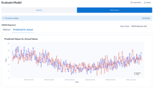
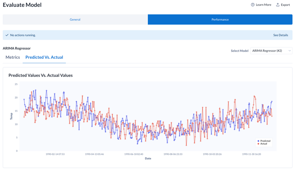
Figure 8: Predicted vs. Actual Values
If we open the “Performance” tab and select “Predicted Vs. Actual,” we can look and see how our predictions on the holdout set, in blue, match up against the actual target values in the holdout set. This is a good quick check to make sure that our model predictions have the same look and feel as the target values and is not generating something like a flat line that would produce great metrics, but zero real world applicability. Ours looks good!
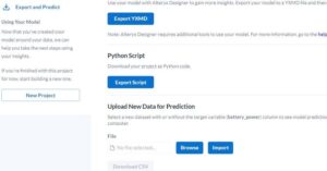
Let’s proceed to the Export and Predict step. At the bottom of the screen are our results in a brand new section!

Figure 9: Time Series Forecast Graph
Our two-week forecast is captured in the Time Series Forecast Graph. The purple extension to our scatterplot represents the projected fourteen days of data off the end of the data we input into the Alteryx Machine Learning. Our charts library lets us hover over the individual data points to get the exact values of our predictions. As before, we can click download graph data to download a .csv file of just the predictions. Also, you’ll notice the presence of prediction intervals, which give us an estimate of the confidence of our predictions and the range in which we statistically expect our predictions to fall.
Well, that ends our tour of some of the new and exciting features added to Alteryx Machine Learning and our time series offering. Trend and seasonality decomposition has greatly enhanced our ability to generate predictive models for time series with additive trend and seasonality. Prediction visualization has further empowered our users to quickly exploit their models for actionable intelligence. With confidence intervals, multiplicative trend and seasonality, and further workflow simplification improvements coming, it’s an exciting time to forecast in Alteryx Machine Learning!