What is time series decomposition?
If you are training a machine learning model for a time series problem and aiming to forecast what may happen in the future – you may notice patterns in your data. The target you’re trying to learn has repeated cycles, and is generally increasing or decreasing over time. For example, sales for a new toy have weekly patterns as more people go out to shop on weekends over weekdays, and the toy is growing in popularity over time. The average temperature in Boston each week fluctuates, but will follow a cycle of warm temperatures in July and cold temperatures in January. The amount of carbon dioxide in the air varies depending on the season thanks to global demand for fossil fuels, but is trending upward as a signal of how our world is growing. In all of these examples, there are micro-patterns amongst the macro-time series.
This is a common occurrence in time series data. There is a clear “trend” to the data, in that it is generally increasing or decreasing over time, and there are “seasons”, or patterns that keep repeating predictably. This is useful information, and can help inform both you and the models you’re training what a reasonable future prediction might be. Time series decomposition “breaks down” the original target data into three separate components: the trend, the seasonality, and the residual, where the residual is simply whatever information is left after removing the trend and seasonality from the data. Training our models on just the residual gives us the opportunity to learn from the unexpected variation in the data, rather than just the expected.
How does decomposition help in EvalML?
We can examine the impacts and insights of decomposition using the carbon dioxide measurements mentioned above. This data is measured once at the start of every month from 1974 to 1986. We can take a look at what the data looks like over time before training our models, as well as get some insight from the decomposed data. To do this, we can run EvalML’s plot_decomposition function:


Here, we can see the original data and its breakdown into separate components. The top graph shows the original data, which is constantly increasing over time while also following a cyclical pattern on a yearly basis. The second and third graphs are that trend and seasonal cycle on their own, and so we are left looking at the other noise as the residual in the fourth graph. This is what we’ll train our forecasting models on, rather than the whole thing. However, we don’t have to worry about doing that ourselves.

Notice with our search call that we don’t have to do anything different than a normal call. Running AutoMLSearch with a time series problem will automatically add this decomposition into the pipelines it trains. However, this sort of decomposition is not always helpful. The example in this post can be very cleanly decomposed into its trend, seasonal, and residual components, but not all data is quite so clean. To guard against cases where decomposition doesn’t work well, we also train models without the decomposition step. This way, we’re testing and directly comparing the performance of each estimator with and without decomposing the data before training, and we can guarantee we’ve tried the more accurate approach.
We can take a look at the pipeline rankings to see how our models performed with and without the time series decomposition step.

Here, since the data was so regular and the decomposition worked well, the pipelines that include decomposition performed much better than those without. We can take a look at the predicted verses actual values of the holdout data to get an idea of the impact of this decomposition.
Here, the best performing model, with decomposition:

Compared to the best performing model that does not use decomposition:

To us as users, we can easily notice seasons and trends in our data and apply them to the future. Traditional machine learning models are not designed for that sort of pattern recognition, as we can see above with the model trained without decomposition. The model has learned that there is a seasonal pattern to the data, but the prediction’s magnitude falls short of the target. When we decompose the target first instead, as with the higher XGBoost model, we have delegated the pattern finding to techniques that are better designed for that purpose. This leaves the model to predict how it does best – picking up the slack where we as users can no longer guess.
Overall, we can see that decomposition significantly improved the forecasting power of our models. By pulling out the patterns within the dataset, we can get valuable insights before even training our models. And once we do, we’ve removed extraneous information so that the models can better optimize for the details of the data.