An explanation and implementation of the first step in solving problems with machine learning.
This is the second in a four-part series on how we approach machine learning at Feature Labs. The set of articles is:
- Overview: A General-Purpose Framework for Machine Learning
- Prediction Engineering (this article)
- Feature Engineering: What Powers Machine Learning
- Modeling: Teaching an Algorithm to Make Predictions
These articles will cover the concepts and a full implementation as applied to predicting customer churn. The project Jupyter Notebooks are all available on GitHub.
Prediction Engineering Concepts
When working with real-world data on a machine learning task, we define the problem, which means we have to develop our own labels — historical examples of what we want to predict — to train a supervised model. The idea of making our own labels may initially seem foreign to data scientists (myself included) who got started on Kaggle competitions or textbook datasets where the answers are already included.
The concept behind prediction engineering — making labels to train a supervised machine learning model — is not new. However, it currently is not a standardized process and is done by data scientists on an as-needed basis. This means that for each new problem — even with the same dataset — a new script must be developed to accomplish this task resulting in solutions that cannot be adapted to different prediction problems.
A better solution is to write functions that are flexible to changing business parameters, allowing us to quickly generate labels for many problems. This is one area where data science can learn from software engineering: solutions should be reusable and accept changing inputs. In this article, we’ll see how to implement a reusable approach to the first step in solving problems with machine learning — prediction engineering.
The Process of Prediction Engineering
Prediction engineering requires guidance both from the business viewpoint to figure out the right problem to solve as well as from the data scientist to determine how to translate the business need into a machine learning problem. The inputs to prediction engineering are the parameters which define the prediction problem for the business requirement , and the historical dataset for finding examples of what we want to predict.
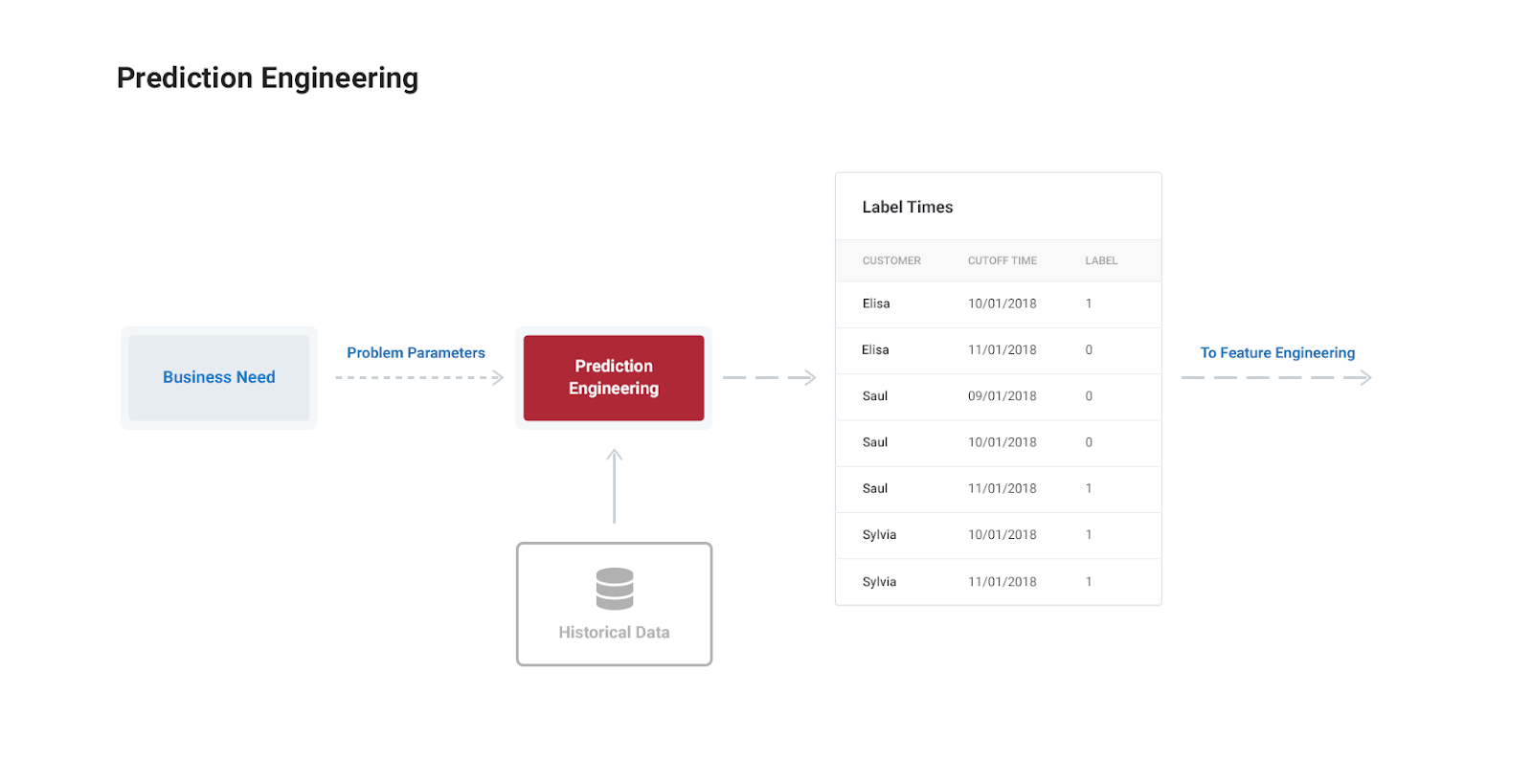
The output of prediction engineering is a label times table: a set of labels with negative and positive examples made from past data along with an associated cutoff time indicating when we have to stop using data to make features for that label (more on this shortly).
For our use case we’ll work through in this series — customer churn — we defined the business problem as increasing monthly active subscribers by reducing rates of churn. The machine learning problem is building a model to predict which customers will churn using historical data. The first step in this task is making a set of labels of past examples of customer churn.
The parameters for what constitutes a churn and how often we want to make predictions will vary depending on the business need, but in this example, let’s say we want to make predictions on the first of each month for which customers will churn one month out from the time of prediction. Churn will be defined as going more than 31 days without an active membership.
It’s important to remember this is only one definition of churn corresponding to one business problem. When we write functions to make labels, they should take in parameters so they can be quickly changed to different prediction problems.
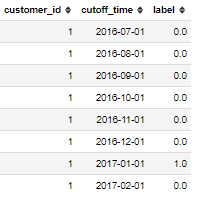
Our goal for prediction engineering is a label times table as follows:
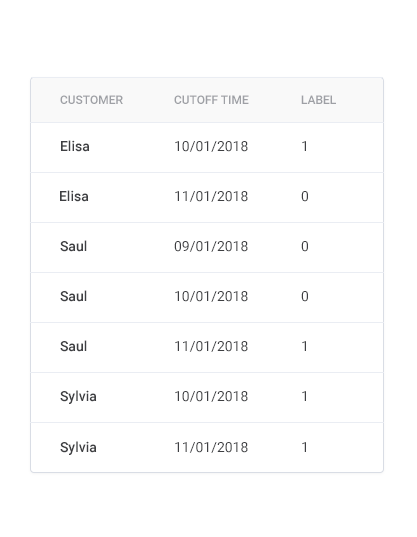
The labels correspond to whether a customer churned or not based on historical data. Each customer is used as a training example multiple times because they have multiple months of data. Even if we didn’t use customers many times, because this is a time-dependent problem, we have to correctly implement the concept of cutoff times.
Cutoff Times: How to Ensure Your Features are Valid
The labels are not complete without the cutoff time which represents when we have to stop using data to make features for a label. Since we are making predictions about customer churn on the first of each month, we can’t use any data after the first to make features for that label. Our cutoff times are therefore all on the first of the month as shown in the label times table above.
All the features for each label must use data from before this time to prevent the problem of data leakage. Cutoff times are a crucial part of building successful solutions to time-series problems that many companies do not account for. Using invalid data to make features leads to models that do well in development but fail in deployment.
Imagine we did not limit our features to data that occurred before the first of the month for each label. Our model would figure out that customers who had a paid transaction during the month could not have churned in that month and would thus record high metrics. However, when it came time to deploy the model and make predictions for a future month, we do not have access to the future transactions and our model would perform poorly. It’s like a student who does great on homework because she has the answer key but then is lost on the test without the same information.
Dataset for Customer Churn
Now that we have the concepts, let’s work go through the details. KKBOX is Asia’s leading music streaming service offering both a free and a pay-per-month subscription option to over 10 million members. KKBOX has made available a dataset for predicting customer churn. There are 3 data tables coming in at just over 30 GB that are represented by the schema below:
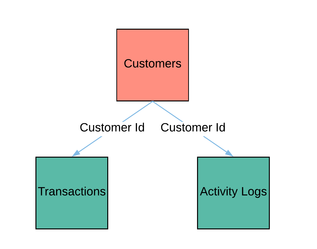
The three tables consist of:
- customers: Background information such as age and city (msno is the customer id):

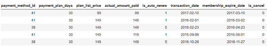
- transactions: Transaction data for each payment for each customer:
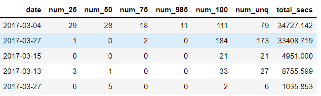
- activity logs: Logs of customer listening behavior:
This is a typical dataset for a subscription business and is an example of structured, relational data: observations in the rows, features in the columns, and tables tied together by primary and foreign keys: the customer id.
Finding Historical Labels
The key to making prediction engineering adaptable to different problems is to follow a repeatable process for extracting training labels from a dataset. At a high-level this is outlined as follows:
- Define positive and negative labels in terms of key business parameters
- Search through past data for positive and negative examples
- Make a table of cutoff times and associate each cutoff time with a label
For customer churn, the parameters are the
- prediction date (cutoff time): the point at which we make a prediction and when we stop using data to make features for the label
- number of days without a subscription before a user is considered a churnlead time: the number of days or months in the future we want to predict
- prediction window: the period of time we want to make predictions for
The following diagram shows each of these concepts while filling in the details with the problem definition we’ll work through.
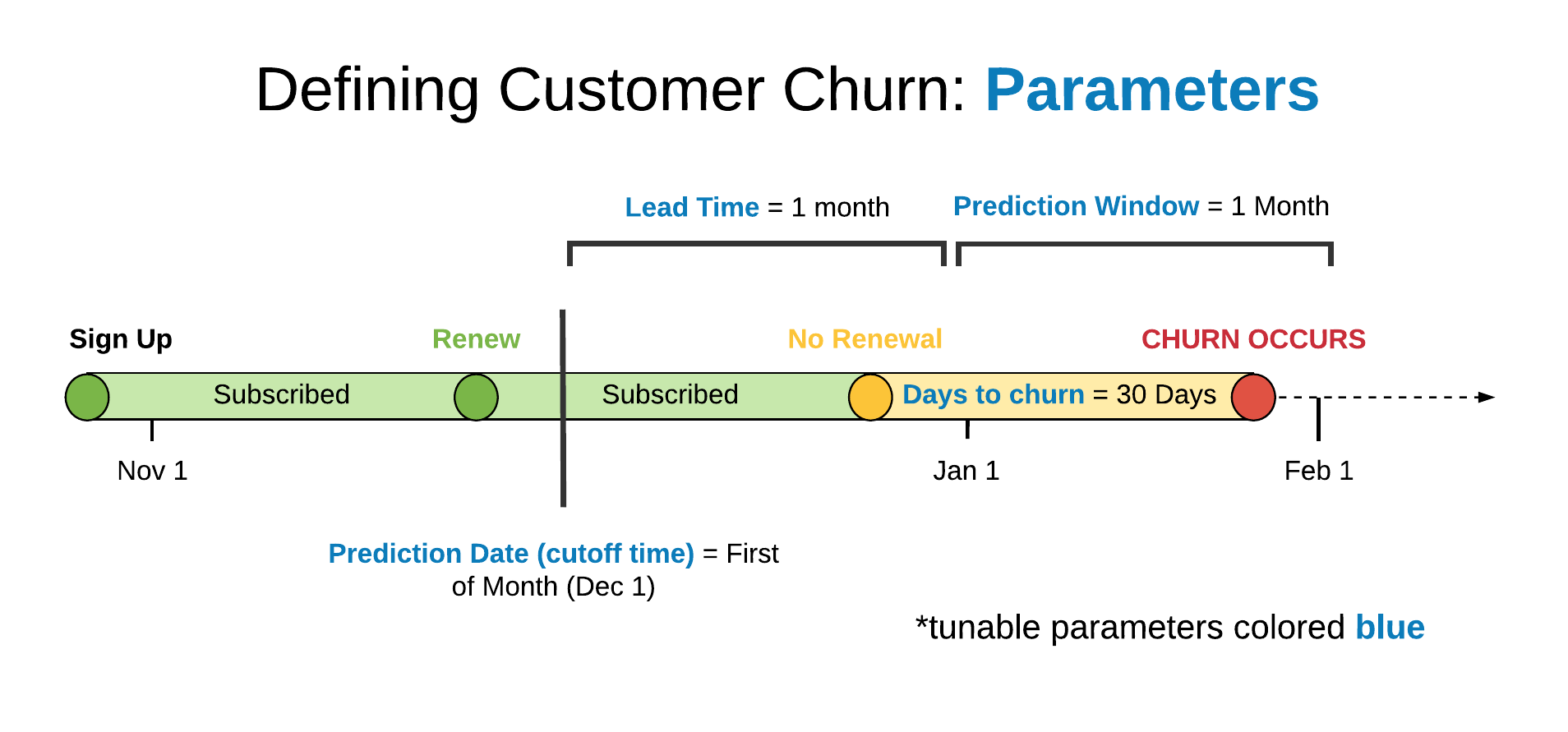
In this case, the customer has churned during the month of January as they went without a subscription for more than 30 days. Because our lead time is one month and the prediction window is also one month, the label of churn is associated with the cutoff time of December 1. For this problem, we are thus teaching our model to predict customer churn one month in advance to give the customer satisfaction team sufficient time to engage with customers.
For a given dataset, there are numerous prediction problems we can make from it. We might want to predict churn at different dates or frequencies, such as every two weeks, with a lead time of two months, or define churn as a shorter duration without an active membership. Moreover, there are other problems unrelated to churn we could solve with this dataset: predict how many songs a customer will listen to in the next month; predict the rate of growth of the customer base; or, segment customers into different groups based on listening habits to tailor a more personal experience.When we develop the functions for creating labels, we make our inputs parameters so we can quickly make multiple sets of labels from the dataset.
If we develop a pipeline that has parameters instead of hard-coded values, we can rapidly adopt it to different problems. When we want to change the definition of a churn, all we need to do is alter the parameter input to our pipeline and re-run it.
Labeling Implementation
To make labels, we develop 2 functions (full code in the notebook):
label_customer(customer_transactions, prediction_date="first of month", days_to_churn = 31, lead_time = "1 month", prediction_window = "1 month")make_labels(all_transactions, prediction_date = "first of month", days_to_churn = 31, lead_time = "1 month", prediction_window = "1 month")The label_customer function takes in a customer’s transactions and the specified parameters and returns a label times table. This table has a set of prediction times — the cutoff times — and the label during the prediction window for each cutoff time corresponding to a single customer.
As an example, our labels for a customer look like the following:
The make_labels function then takes in the transactions for all customers along with the parameters and returns a table with the cutoff times and the label for every customer.
Next Steps
When implemented correctly, the end outcome of prediction engineering is a function which can create label times for multiple prediction problems by changing input parameters. These labels times — a cutoff time and associated label — are the input to the next stage in which we make features for each label. The next article in the series describes how feature engineering works .
Conclusion
We haven’t invented the process of prediction engineering, just given it a name and defined a reusable approach for this first part in the pipeline.The process of prediction engineering is captured in three steps:
- Identify a business need that can be solved with available data
- Translate the business need into a supervised machine learning problem
- Create label times from historical data
Getting prediction engineering right is crucial and requires input from both the business and data science sides of a business. By writing the code for prediction engineering to accept different parameters, we can rapidly change the prediction problem if the needs of our company change.
More generally, our approach to solving problems with machine learning segments the different parts of the pipeline while standardizing each input and output. The end result, as we’ll see, is we can quickly change the prediction problem in the prediction engineering stage without needing to rewrite the subsequent steps. In this article, we’ve developed the first step in a framework that can be used to solve many problems with machine learning.
If building meaningful, high-performance predictive models is something you care about, then get in touch with us at Feature Labs. While this project was completed with the open-source Featuretools, the commercial product offers additional tools and support for creating machine learning solutions.