Automated feature engineering will save you time, build better predictive models, create meaningful features, and prevent data leakage
There are few certainties in data science — libraries, tools, and algorithms constantly change as better methods are developed. However, one trend that is not going away is the move towards increased levels of automation.
Recent years have seen progress in automating model selection and hyperparameter tuning, but the most important aspect of the machine learning pipeline, feature engineering, has largely been neglected. The most capable entry in this critical field is Featuretools, an open-source Python library. In this article, we’ll use this library to see how automated feature engineering will change the way you do machine learning for the better.

Automated feature engineering is a relatively new technique, but, after using it to solve a number of data science problems using real-world data sets, I’m convinced it should be a standard part of any machine learning workflow. Here we’ll take a look at the results and conclusions from two of these projects with the full code available as Jupyter Notebooks on GitHub.
Each project highlights some of the benefits of automated feature engineering:
- Loan Repayment Prediction: automated feature engineering can reduce machine learning development time by 10x compared to manual feature engineering while delivering better modeling performance. (Notebooks)
- Retail Spending Prediction: automated feature engineering creates meaningful features and prevents data leakage by internally handling time-series filters, enabling successful model deployment. (Notebooks)
Feature Engineering: Manual vs. Automated
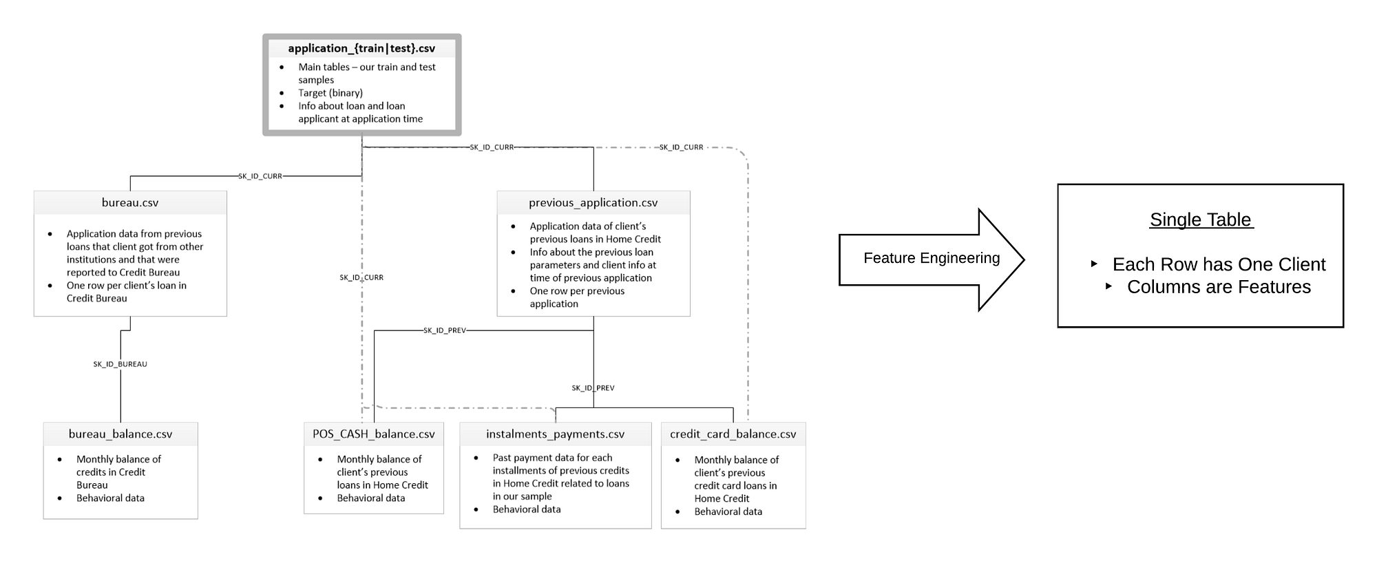
Feature engineering is the process of taking a dataset and constructing explanatory variables — features — that can be used to train a machine learning model for a prediction problem. Often, data is spread across multiple tables and must be gathered into a single table with rows containing the observations and features in the columns.
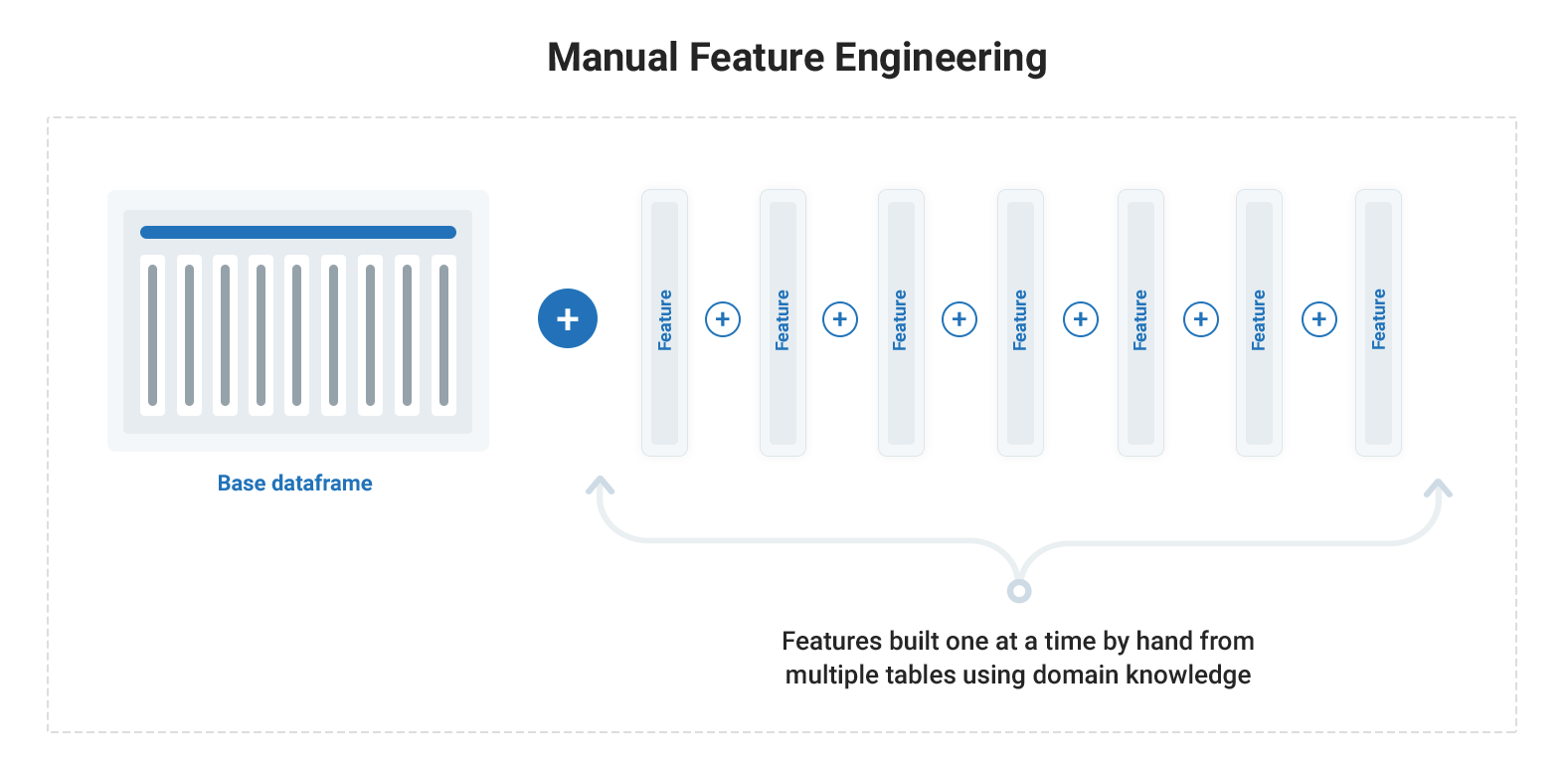
The traditional approach to feature engineering is to build features one at a time using domain knowledge, a tedious, time-consuming, and error-prone process known as manual feature engineering. The code for manual feature engineering is problem-dependent and must be re-written for each new dataset.
Automated feature engineering improves upon this standard workflow by automatically extracting useful and meaningful features from a set of related data tables with a framework that can be applied to any problem. It not only cuts down on the time spent feature engineering, but creates interpretable features and prevents data leakage by filtering time-dependent data.
Automated feature engineering is more efficient and repeatable than manual feature engineering allowing you to build better predictive models faster.
Loan Repayment: Build Better Models Faster
The primary difficulty facing a data scientist approaching the Home Credit Loan problem (a machine learning competition currently running on Kagglewhere the objective is to predict if a loan will be repaid by a client) is the size and spread of the data. Take a look at the complete dataset and you are confronted with 58 million rows of data spread across seven tables. Machine learning requires a single table for training, so feature engineering means consolidating all the information about each client in one table.
My first attempt at the problem used traditional manual feature engineering: I spent a total of 10 hours creating a set of features by hand. First I read other data scientist’s work, explored the data, and researched the problem area in order to acquire the necessary domain knowledge. Then I translated the knowledge into code, building one feature at a time. As an example of a single manual feature, I found the total number of late payments a client had on previous loans, an operation that required using 3 different tables.
The final manual engineered features performed quite well, achieving a 65% improvement over the baseline features (relative to the top leaderboard score), indicating the importance of proper feature engineering.
However, inefficient does not even begin to describe this process. For manual feature engineering, I ended up spending over 15 minutes per feature because I used the traditional approach of making a single feature at a time.
Besides being tedious and time-consuming, manual feature engineering is:
- Problem-specific: all of the code I wrote over many hours cannot be applied to any other problem
- Error-prone: each line of code is another opportunity to make a mistake
Retail Spending: Build Meaningful Features and Prevent Data Leakage
For the second dataset, a record of online time-stamped customer transactions, the prediction problem is to classify customers into two segments, those who will spend more than $500 in the next month and those who won’t. However, instead of using a single month for all the labels, each customer is a label multiple times. We can use their spending in May as a label, then in June, and so on.
Using each customer multiple times as an observation brings up difficulties for creating training data: when making features for a customer for a given month, we can’t use any information from months in the future, even though we have access to this data. In a deployment, we’ll never have future data and therefore can’t use it for training a model. Companies routinely struggle with this issue and often deploy a model that does much worse in the real world than in development because it was trained using invalid data.
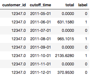
Fortunately, ensuring that our data is valid in a time-series problem is straightforward in Featuretools. In the Deep Feature Synthesis function we pass in a dataframe like that shown above, where the cutoff time represents the point past which we can’t use any data for the label, and Featuretools automatically takes the time into account when building features.
The features for a customer in a given month are built using data filtered to before the month. Notice that the call to create our set of features is the same as that for the loan repayment problem with the addition of cutoff_time.
# Deep feature synthesisfeature_matrix, features = ft.dfs(entityset=es, target_entity='customers', agg_primitives = agg_primitives, trans_primitives = trans_primitives, cutoff_time = cutoff_times)The result of running Deep Feature Synthesis is a table of features, one for each customer for each month. We can use these features to train a model with our labels and then make predictions for any month. Moreover, we can rest assured that the features in our model do not use future information, which would result in an unfair advantage and yield misleading training scores.
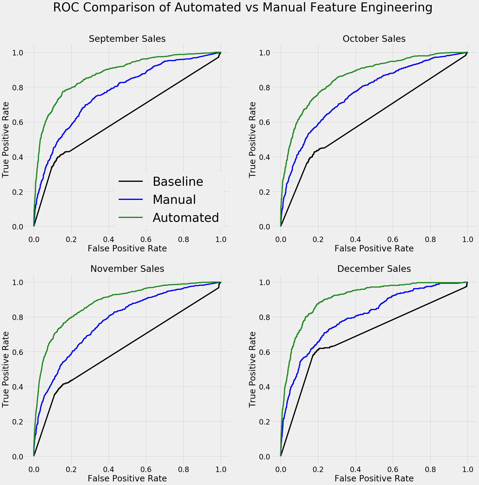
With the automated features, I was able to build a machine learning model that achieved 0.90 ROC AUC compared to an informed baseline (guessing the same level of spending as the previous month) of 0.69 when predicting customer spending categories for one month.
In addition to delivering impressive predictive performance, the Featuretools implementation gave me something equally valuable: interpretable features. Take a look at the 15 most important features from a random forest model:
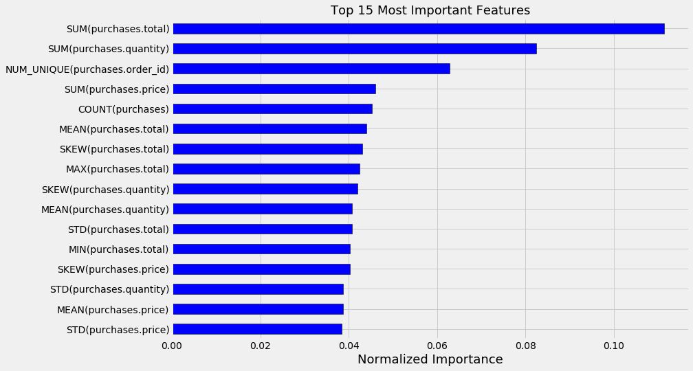
The feature importances tell us that the most important predictors of how much the customer will spend in the next month is how much they have spent previously SUM(purchases.total) , and the number of purchases, SUM(purchases.quantity).These are features that we could have built by hand, but then we would have to worry about leaking data and creating a model that does much better in development than in deployment.
If the tool already exists for creating meaningful features without any need to worry about the validity of our features, then why do the implementation by hand? Furthermore, the automated features are completely clear in the context of the problem and can inform our real-world reasoning.
Automated feature engineering identified the most important signals, achieving the primary goal of data science: reveal insights hidden in mountains of data.
Even after spending significantly more time on manual feature engineering than I did with Featuretools, I was not able to develop a set of features with close to the same performance. The graph below shows the ROC curves for classifying one month of future customer sales using a model trained on the two datasets. A curve to the left and top indicates better predictions:
I’m not even completely sure if the manual features were made using valid data, but with the Featuretools implementation, I didn’t have to worry about data leakage in time-dependent problems. Maybe this inability to manually engineer a useful set of valid features speaks to my failings as a data scientist, but if the tool exists to safely do this for us, why not use it?
We use automatic safety systems in our day-to-day life and automated feature engineering in Featuretools is the secure method to build meaningful machine learning features in a time-series problem while delivering superior predictive performance.
Conclusions
I came away from these projects convinced that automated feature engineering should be an integral part of the machine learning workflow. The technology is not perfect yet still delivers significant gains in efficiency.
The main conclusions are that automated feature engineering:
- Reduced implementation time by up to 10x
- Achieved modeling performance at the same level or better
- Delivered interpretable features with real-world significance
- Prevented improper data usage that would invalidate a model
- Fit into existing workflows and machine learning models